pypose.module.IMUPreintegrator
- class pypose.module.IMUPreintegrator(pos=tensor([0., 0., 0.]), rot=SO3Type LieTensor: LieTensor([0., 0., 0., 1.]), vel=tensor([0., 0., 0.]), gravity=9.81007, gyro_cov=1.024e-05, acc_cov=0.0064, prop_cov=True, reset=False)[source]
Applies preintegration over IMU input signals.
- Parameters
pos (torch.Tensor, optional) – initial position. Default:
torch.zeros(3).rot (pypose.SO3, optional) – initial rotation. Default:
pypose.identity_SO3().vel (torch.Tensor, optional) – initial position. Default: torch.zeros(3).
gravity (float, optional) – the gravity acceleration. Default: 9.81007.
gyro_cov – covariance of the gyroscope. Default: (3.2e-3)**2. Use the form
torch.Tensor(gyro_cov_x, gyro_cov_y, gyro_cov_z), if the covariance on the three axes are different.acc_cov – covariance of the accelerator. Default: (8e-2)**2. Use the form
torch.Tensor(acc_cov_x, acc_cov_y,acc_cov_z), if the covariance on the three axes are different.prop_cov (Bool, optional) – flag to propagate the covariance matrix. Default:
True.reset (Bool, optional) – flag to reset the initial states after the
forwardfunction is called. IfFalse, the integration starts from the last integration. This flag is ignored ifinit_stateis notNone. Default:False.
- forward(dt, gyro, acc, rot=None, gyro_cov=None, acc_cov=None, init_state=None)[source]
Propagate IMU states from duration (\(\delta t\)), gyroscope (angular rate \(\omega\)), linear acceleration (\(\mathbf{a}\)) in body frame, as well as their measurement covariance for gyroscope \(C_{g}\) and acceleration \(C_{\mathbf{a}}\). Known IMU rotation estimation \(R\) can be provided for better precision.
- Parameters
dt (torch.Tensor) – time interval from last update.
gyro (torch.Tensor) – angular rate (\(\omega\)) in IMU body frame.
acc (torch.Tensor) – linear acceleration (\(\mathbf{a}\)) in IMU body frame (raw sensor input with gravity).
rot (
pypose.SO3, optional) – known IMU rotation.gyro_cov (torch.Tensor, optional) – covariance matrix of angular rate. If not given, the default state in constructor will be used.
acc_cov (torch.Tensor, optional) – covariance matrix of linear acceleration. If not given, the default state in constructor will be used.
init_state (Dict, optional) – the initial state of the integration. The dictionary should be in form of
{'pos': torch.Tensor, 'rot': pypose.SO3, 'vel':
torch.Tensor}
. If not given, the initial state in constructor will be used.
- Shape:
input (
dt,gyro,acc): This layer supports the input shape with \((B, F, H_{in})\), \((F, H_{in})\) and \((H_{in})\), where \(B\) is the batch size (or the number of IMU), \(F\) is the number of frames (measurements), and \(H_{in}\) is the raw sensor signals.init_state (Optional): The initial state of the integration. It contains
pos: initial position,rot: initial rotation,vel: initial velocity, with the shape \((B, H_{in})\)output: a
dictof integrated state includingpos: position,rot: rotation, andvel: velocity, each of which has a shape \((B, F, H_{out})\), where \(H_{out}\) is the signal dimension. Ifprop_covisTrue, it will also includecov: covariance matrix in shape of \((B, 9, 9)\).
IMU Measurements Integration:
\[\begin{align*} {\Delta}R_{ik+1} &= {\Delta}R_{ik} \mathrm{Exp} (w_k {\Delta}t) \\ {\Delta}v_{ik+1} &= {\Delta}v_{ik} + {\Delta}R_{ik} a_k {\Delta}t \\ {\Delta}p_{ik+1} &= {\Delta}p_{ik} + {\Delta}v_{ik} {\Delta}t + \frac{1}{2} {\Delta}R_{ik} a_k {\Delta}t^2 \end{align*} \]where:
\({\Delta}R_{ik}\) is the preintegrated rotation between the \(i\)-th and \(k\)-th time step.
\({\Delta}v_{ik}\) is the preintegrated velocity between the \(i\)-th and \(k\)-th time step.
\({\Delta}p_{ik}\) is the preintegrated position between the \(i\)-th and \(k\)-th time step.
\(a_k\) is linear acceleration at the \(k\)-th time step.
\(w_k\) is angular rate at the \(k\)-th time step.
\({\Delta}t\) is the time interval from time step \(k\)-th to time step \({k+1}\)-th time step.
Uncertainty Propagation:
\[\begin{align*} C_{ik+1} &= A C_{ik} A^T + B \mathrm{diag}(C_g, C_a) B^T \\ &= A C A^T + B_g C_g B_g^T + B_a C_a B_a^T \end{align*}, \]where
\[A = \begin{bmatrix} {\Delta}R_{ik+1}^T & 0_{3*3} \\ -{\Delta}R_{ik} (a_k^{\wedge}) {\Delta}t & I_{3*3} & 0_{3*3} \\ -1/2{\Delta}R_{ik} (a_k^{\wedge}) {\Delta}t^2 & I_{3*3} {\Delta}t & I_{3*3} \end{bmatrix}, \]\[B = [B_g, B_a] \\ \]\[B_g = \begin{bmatrix} J_r^k \Delta t \\ 0_{3*3} \\ 0_{3*3} \end{bmatrix}, B_a = \begin{bmatrix} 0_{3*3} \\ {\Delta}R_{ik} {\Delta}t \\ 1/2 {\Delta}R_{ik} {\Delta}t^2 \end{bmatrix},\]where \(\cdot^\wedge\) is the skew matrix (
pypose.vec2skew()), \(C \in\mathbf{R}^{9\times 9}\) is the covariance matrix, and \(J_r^k\) is the right jacobian (pypose.Jr()) of integrated rotation \(\mathrm{Exp}(w_k{\Delta}t)\) at \(k\)-th time step, \(C_{g}\) and \(C_{\mathbf{a}}\) are measurement covariance of angular rate and acceleration, respectively.Note
Output covariance (Shape: \((B, 9, 9)\)) is in the order of rotation, velocity, and position.
With IMU preintegration, the propagated IMU status:
\[\begin{align*} R_j &= {\Delta}R_{ij} * R_i \\ v_j &= R_i * {\Delta}v_{ij} + v_i + g \Delta t_{ij} \\ p_j &= R_i * {\Delta}p_{ij} + p_i + v_i \Delta t_{ij} + 1/2 g \Delta t_{ij}^2 \\ \end{align*} \]where:
\({\Delta}R_{ij}\), \({\Delta}v_{ij}\), \({\Delta}p_{ij}\) are the preintegrated measurements.
\(R_i\), \(v_i\), and \(p_i\) are the initial state. Default initial values are used if
resetis True.\(R_j\), \(v_j\), and \(p_j\) are the propagated state variables.
\({\Delta}t_{ij}\) is the time interval from frame i to j.
Note
The implementation is based on Eq. (A7), (A8), (A9), and (A10) of this report:
Christian Forster, et al., IMU Preintegration on Manifold for Efficient Visual-Inertial Maximum-a-posteriori Estimation, Technical Report GT-IRIM-CP&R-2015-001, 2015.
Example
Preintegrator Initialization
>>> import torch
>>> import pypose as pp
>>> p = torch.zeros(3)    # Initial Position
>>> r = pp.identity_SO3() # Initial rotation
>>> v = torch.zeros(3)    # Initial Velocity
>>> integrator = pp.module.IMUPreintegrator(p, r, v)
Get IMU measurement
>>> ang = torch.tensor([0.1,0.1,0.1]) # angular velocity
>>> acc = torch.tensor([0.1,0.1,0.1]) # acceleration
>>> rot = pp.mat2SO3(torch.eye(3))    # Rotation (Optional)
>>> dt = torch.tensor([0.002])        # Time difference between two measurements
3. Preintegrating IMU measurements. Takes as input the IMU values and calculates the preintegrated IMU measurements.
>>> states = integrator(dt, ang, acc, rot)
{'rot': SO3Type LieTensor:
tensor([[[1.0000e-04, 1.0000e-04, 1.0000e-04, 1.0000e+00]]]),
'vel': tensor([[[ 0.0002,  0.0002, -0.0194]]]),
'pos': tensor([[[ 2.0000e-07,  2.0000e-07, -1.9420e-05]]]),
'cov': tensor([[[ 5.7583e-11, -5.6826e-19, -5.6827e-19,  0.0000e+00,  0.0000e+00,
                  0.0000e+00,  0.0000e+00,  0.0000e+00,  0.0000e+00],
                [-5.6826e-19,  5.7583e-11, -5.6827e-19,  0.0000e+00,  0.0000e+00,
                  0.0000e+00,  0.0000e+00,  0.0000e+00,  0.0000e+00],
                [-5.6827e-19, -5.6827e-19,  5.7583e-11,  0.0000e+00,  0.0000e+00,
                  0.0000e+00,  0.0000e+00,  0.0000e+00,  0.0000e+00],
                [ 0.0000e+00,  0.0000e+00,  0.0000e+00,  8.0000e-09, -3.3346e-20,
                 -1.0588e-19,  8.0000e-12,  1.5424e-23, -1.0340e-22],
                [ 0.0000e+00,  0.0000e+00,  0.0000e+00, -1.3922e-19,  8.0000e-09,
                  0.0000e+00, -8.7974e-23,  8.0000e-12,  0.0000e+00],
                [ 0.0000e+00,  0.0000e+00,  0.0000e+00,  0.0000e+00, -1.0588e-19,
                  8.0000e-09,  0.0000e+00, -1.0340e-22,  8.0000e-12],
                [ 0.0000e+00,  0.0000e+00,  0.0000e+00,  8.0000e-12,  1.5424e-23,
                 -1.0340e-22,  8.0000e-15, -1.2868e-26,  0.0000e+00],
                [ 0.0000e+00,  0.0000e+00,  0.0000e+00, -8.7974e-23,  8.0000e-12,
                  0.0000e+00, -1.2868e-26,  8.0000e-15,  0.0000e+00],
                [ 0.0000e+00,  0.0000e+00,  0.0000e+00,  0.0000e+00, -1.0340e-22,
                  8.0000e-12,  0.0000e+00,  0.0000e+00,  8.0000e-15]]])}
Preintegrated IMU odometry from the KITTI dataset with and without known rotation.
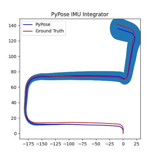
Fig. 1. Known Rotation.
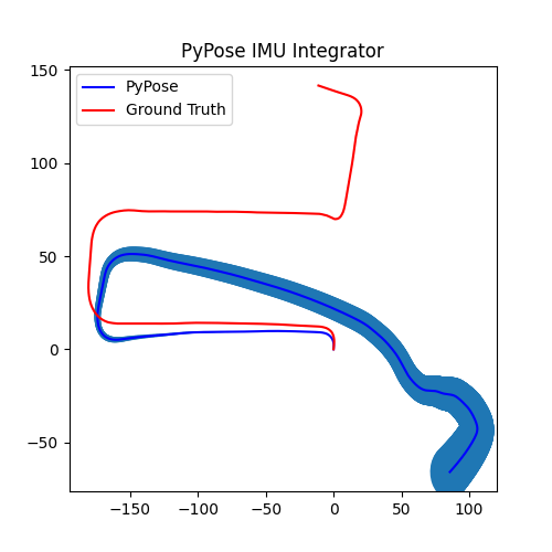
Fig. 2. Estimated Rotation.
Note
The examples generating the above figures can be found at examples/module/imu.
