Cartpole Tutorial

import torch, pypose as pp
import math, matplotlib.pyplot as plt

device = torch.device("cuda" if torch.cuda.is_available() else "cpu")

Preparation

Create class for cart-pole dynamics

class CartPole(pp.module.NLS):
    def __init__(self, dt, length, cartmass, polemass, gravity):
        super().__init__()
        self.tau = dt
        self.length = length
        self.cartmass = cartmass
        self.polemass = polemass
        self.gravity = gravity
        self.polemassLength = self.polemass * self.length
        self.totalMass = self.cartmass + self.polemass

    def state_transition(self, state, input, t = None):
        x, xDot, theta, thetaDot = state
        force = input.squeeze()
        costheta = theta.cos()
        sintheta = theta.sin()

        temp = (force + self.polemassLength * thetaDot**2 * sintheta) / self.totalMass

        thetaAcc = (self.gravity * sintheta - costheta * temp) / \
            (self.length * (4.0 / 3.0 - self.polemass * costheta**2 / self.totalMass))

        xAcc = temp - self.polemassLength * thetaAcc * costheta / self.totalMass

        _dstate = torch.stack((xDot, xAcc, thetaDot, thetaAcc))

        return state + _dstate * self.tau

    def observation(self, state, input, t = None):
        return state


def subPlot(ax, x, y, xlabel=None, ylabel=None):
    x = x.detach().cpu().numpy()
    y = y.detach().cpu().numpy()
    ax.plot(x, y)
    ax.set_xlabel(xlabel)
    ax.set_ylabel(ylabel)

Create parameters for cart pole trajectory

dt = 0.01   # Delta t
len = 1.5   # Length of pole
m_cart = 20 # Mass of cart
m_pole = 10 # Mass of pole
g = 9.81    # Accerleration due to gravity
N = 1000    # Number of time steps

Time and input

time  = torch.arange(0, N, device=device) * dt
input = torch.sin(time)

Initial state

state = torch.zeros(N, 4, dtype=float, device=device)
state[0] = torch.tensor([0, 0, math.pi, 0], dtype=float, device=device)

Create dynamics solver object

model = CartPole(dt, len, m_cart, m_pole, g).to(device)

Calculate trajectory

for i in range(N - 1):
    state[i + 1], _ = model(state[i], input[i])

Jacobian computation - Find jacobians at the last step

model.set_refpoint(state=state[-1,:], input=input[-1], t=time[-1])
vars = ['A', 'B', 'C', 'D', 'c1', 'c2']
[print(v, getattr(model, v)) for v in vars]

A tensor([[ 1.0000e+00,  1.0000e-02,  0.0000e+00,  0.0000e+00],
        [ 0.0000e+00,  1.0000e+00, -3.2700e-02, -3.4183e-07],
        [ 0.0000e+00,  0.0000e+00,  1.0000e+00,  1.0000e-02],
        [ 0.0000e+00,  0.0000e+00, -6.5400e-02,  1.0000e+00]], device='cuda:0',
       dtype=torch.float64)
B tensor([[0.0000],
        [0.0004],
        [0.0000],
        [0.0002]], device='cuda:0')
C tensor([[1., 0., 0., 0.],
        [0., 1., 0., 0.],
        [0., 0., 1., 0.],
        [0., 0., 0., 1.]], device='cuda:0', dtype=torch.float64)
D tensor([[0.],
        [0.],
        [0.],
        [0.]], device='cuda:0')
c1 tensor([0.0000, 0.1027, 0.0000, 0.2055], device='cuda:0', dtype=torch.float64)
c2 tensor([0., 0., 0., 0.], device='cuda:0', dtype=torch.float64)

[None, None, None, None, None, None]

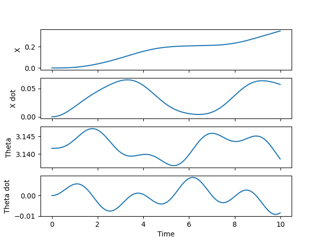
Create time plots to show dynamics

f, ax = plt.subplots(nrows=4, sharex=True)
x, xdot, theta, thetadot = state.T
subPlot(ax[0], time, x, ylabel='X')
subPlot(ax[1], time, xdot, ylabel='X dot')
subPlot(ax[2], time, theta, ylabel='Theta')
subPlot(ax[3], time, thetadot, ylabel='Theta dot', xlabel='Time')
plt.show()