Floquet Tutorial

import torch, pypose as pp
import math, matplotlib.pyplot as plt

device = torch.device("cuda" if torch.cuda.is_available() else "cpu")

Preparation

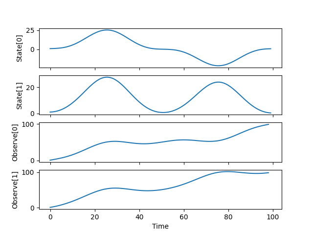
We consider a Floquet system, which is periodic and an example of time-varying systems

class Floquet(pp.module.NLS):
    '''
    Floquet system is periodic and time-varying.
    '''
    def __init__(self):
        super().__init__()

    def state_transition(self, state, input, t):
        cc = (2 * math.pi * t / 100).cos()
        ss = (2 * math.pi * t / 100).sin()
        A = torch.tensor([[   1.,  cc/10],
                          [cc/10,     1.]], device=t.device)
        B = torch.tensor([[ss],
                          [1.]], device=t.device)

        return A @ state + B @ input

    def observation(self, state, input, t):
        return state + t


def subPlot(ax, x, y, xlabel=None, ylabel=None):
    x = x.detach().cpu().numpy()
    y = y.detach().cpu().numpy()
    ax.plot(x, y)
    ax.set_xlabel(xlabel)
    ax.set_ylabel(ylabel)

Number of time steps

N = 100

Time, Input, Initial state

time  = torch.arange(0, N, device=device)
input = (2 * math.pi * time / 50).sin()

state = torch.zeros(N, 2, device=device)
state[0] = torch.tensor([1., 1.], device=device)
obser = torch.zeros(N, 2, device=device)

Create dynamics solver object

model = Floquet().to(device)

Calculate trajectory

for i in range(N - 1):
    state[i + 1], obser[i] = model(state[i], input[i])

Jacobian computation - Find jacobians at the last step

vars = ['A', 'B', 'C', 'D', 'c1', 'c2']
model.set_refpoint()
[print(v, getattr(model, v)) for v in vars]

A tensor([[1.0000, 0.0998],
        [0.0998, 1.0000]], device='cuda:0')
B tensor([[-0.0628],
        [ 1.0000]], device='cuda:0')
C tensor([[1., 0.],
        [0., 1.]], device='cuda:0')
D tensor([[0.],
        [0.]], device='cuda:0')
c1 tensor([ 2.9802e-08, -1.4901e-08], device='cuda:0')
c2 tensor([99., 99.], device='cuda:0')

[None, None, None, None, None, None]

Jacobian computation - Find jacobians at the 5th step

idx = 5
model.set_refpoint(state=state[idx], input=input[idx], t=time[idx])
[print(v, getattr(model, v)) for v in vars]

A tensor([[1.0000, 0.0951],
        [0.0951, 1.0000]], device='cuda:0')
B tensor([[0.3090],
        [1.0000]], device='cuda:0')
C tensor([[1., 0.],
        [0., 1.]], device='cuda:0')
D tensor([[0.],
        [0.]], device='cuda:0')
c1 tensor([-1.4901e-08,  0.0000e+00], device='cuda:0')
c2 tensor([5., 5.], device='cuda:0')

[None, None, None, None, None, None]

Create time plots to show dynamics

f, ax = plt.subplots(nrows=4, sharex=True)
subPlot(ax[0], time, state[:, 0], ylabel='State[0]')
subPlot(ax[1], time, state[:, 1], ylabel='State[1]')
subPlot(ax[2], time[:-1], obser[:-1, 0], ylabel='Observe[0]')
subPlot(ax[3], time[:-1], obser[:-1, 1], ylabel='Observe[1]', xlabel='Time')
plt.show()